Using the scikit-learn library
Contents
Using the scikit-learn library
from sklearn.datasets import make_blobs, make_classification
import matplotlib.pyplot as plt
import pandas as pd
The scikit-learn library contains functions for generating random numeric datasets that can be used for classification or regression. The previous chapter made use of numpy to generate arrays of data. In this chapter, we’ll find that scikit-learn also makes use of numpy to generate data, but its implementation is abstracted by functions that output multi-dimensional arrays with specific characteristics. We can then make use of a library called pandas to convert these arrays into a dataframe, which allows us to operate on the data as matrices.
The datasets module contains these handy data generation functions.
Generating data for classification
Using make_blobs()
Scikit-learn’s make_blob() function generates random datasets of a gaussian distribution (technically a guassian mixture), where you can specify the number of samples (through n_samples) and the number of clusters (through centers).
In the example below, we generate 10,000 samples grouped into 4 clusters. make_blobs() outputs two things: the random array of features and the labels. Here we store the features in X and the labels in y.
# Generate 10,000 samples with 2 features and 4 possible labels
X, y = make_blobs(n_samples=10000, centers=4, n_features=2)
As mentioned earlier, scikit-learn utilises numpy under the hood. We can check that by looking at the type of the generated data in X and y.
print('Type of X:', type(X))
print('Type of y:', type(y))
Type of X: <class 'numpy.ndarray'>
Type of y: <class 'numpy.ndarray'>
We can then structure X and y as a dataframe. We’ve specified n_features=2 above, so X has two columns. We’ll name the columns a and b in this example.
# Structure X and y as a dataframe
df = pd.DataFrame(dict(a=X[:,0],  b=X[:,1], label=y))
We can preview df to check its size and columns.
df
| a | b | label | |
|---|---|---|---|
| 0 | 1.754258 | -8.309663 | 2 |
| 1 | -8.865031 | 5.164420 | 1 |
| 2 | -1.141462 | 0.090764 | 0 |
| 3 | -7.748770 | 6.245700 | 1 |
| 4 | -6.133729 | 7.027466 | 1 |
| ... | ... | ... | ... |
| 9995 | 0.992074 | -8.043875 | 2 |
| 9996 | 2.252391 | -8.540260 | 2 |
| 9997 | 1.482460 | -8.961066 | 2 |
| 9998 | -0.199096 | -3.018672 | 0 |
| 9999 | -3.120199 | 4.527252 | 3 |
10000 rows × 3 columns
To check the number of unique labels (i.e., the clusters), we can use the unique() function of the dataframe object. We’ll see that since we’ve specified that there are 4 clusters, then there should 4 unique values as the data labels.
df['label'].unique()
array([2, 1, 0, 3])
Plotting the dataframe, we can easily make sense of the generated clusters. Here we’ve provided y as the value of the parameter c, which is a list of colors to assign to each cluster. By default pyplot does that for us using the size of c to get the number of colors to use. The s parameter is just the thickness of each data point on the plot.
plt.scatter(df['a'], df['b'], c=y, s=2)
<matplotlib.collections.PathCollection at 0x14d4b6940>
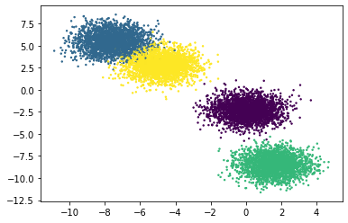
We can see that the clusters are easily linearly separable. The make_blobs() function is suitable for testing linear models.
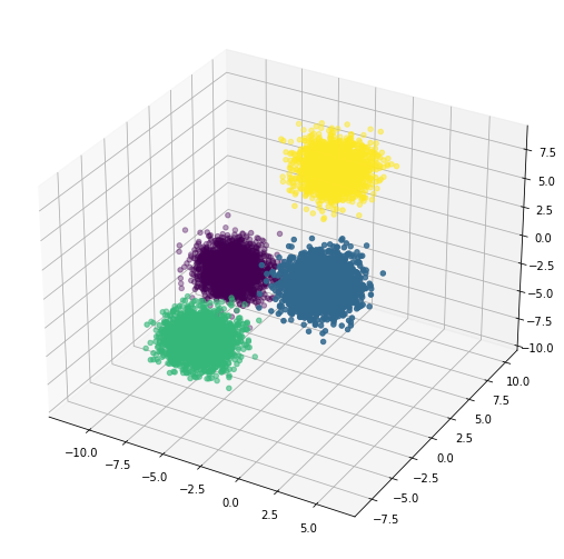
We can easily add more features into the dataset by specifying the number in the n_features parameter. Here we reuse the code above and add 1 new feature which we’ll name c, and then visualise the generated data in a 3D scatter plot. Notice again that the data clusters are linearly separable by a 2D plane.
# 3 features and 4 possible labels
X, y = make_blobs(n_samples=10000, centers=4, n_features=3)
df = pd.DataFrame(dict(a=X[:,0],  b=X[:,1], c=X[:,2], label=y))

fig = plt.figure(figsize = (10, 9))
ax = plt.axes(projection ="3d")
ax.scatter3D(df['a'], df['b'], df['c'], c=y)
<mpl_toolkits.mplot3d.art3d.Path3DCollection at 0x14d5e56a0>
A more powerful way: make_classification()
# Normal data
X, y = make_classification(n_samples=10000,
                           n_features=2,
                           n_informative=2,
                           n_redundant=0,
                           n_repeated=0,
                           n_classes=3,
                           n_clusters_per_class=1,
                           class_sep=2,
                           flip_y=0,
                           weights=[0.3,0.3,0.3],
                           random_state=13,
                          )
df = pd.DataFrame(dict(a=X[:,0], b=X[:,1],label=y))
plt.scatter(df['a'], df['b'], c=y, s=2)
<matplotlib.collections.PathCollection at 0x14d6a2ee0>
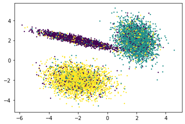
# Noisy data
X, y = make_classification(n_samples=10000,
                           n_features=2,
                           n_informative=2,
                           n_redundant=0,
                           n_repeated=0,
                           n_classes=3,
                           n_clusters_per_class=1,
                           class_sep=2,
                           flip_y=0.3,   # 30% noise?
                           weights=[0.3,0.3,0.3],
                           random_state=13,
                          )
df = pd.DataFrame(dict(a=X[:,0], b=X[:,1],label=y))
plt.scatter(df['a'], df['b'], c=y, s=2)
<matplotlib.collections.PathCollection at 0x14d716220>
# Imbalanced data
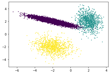
X, y = make_classification(n_samples=10000,
                           n_features=2,
                           n_informative=2,
                           n_redundant=0,
                           n_repeated=0,
                           n_classes=3,
                           n_clusters_per_class=1,
                           class_sep=2,
                           flip_y=0,
                           weights=[0.8,0.1,0.1],  # one cluster is 80% of the data
                           random_state=13,
                          )
df = pd.DataFrame(dict(a=X[:,0], b=X[:,1],label=y))
plt.scatter(df['a'], df['b'], c=y, s=2)
<matplotlib.collections.PathCollection at 0x14d75ee80>
# Redundant data
X, y = make_classification(n_samples=10000,
                           n_features=4,
                           n_informative=1,
                           n_redundant=3,
                           n_repeated=0,
                           n_classes=2,
                           n_clusters_per_class=1,
                           class_sep=2,
                           flip_y=0,
#                            weights=[0.3,0.3,0.3],
                           random_state=13,
                          )
df = pd.DataFrame(dict(a=X[:,0], b=X[:,1],label=y))
plt.scatter(df['a'], df['b'], c=y, s=2)
<matplotlib.collections.PathCollection at 0x14d7c7760>
